Linear Regression with Matlab Using Batch Gradient Descent Algorithm

i will implement linear regression which can be adapted classification easily,  i use Matlab by following the  Dr. Andrew Ng's class. You can watch the classes online from here.

While implementing i also came across a very nice blog post, actually only dataset differs, in this case i use the original dataset given by the Dr. Ng, more details of the code below can be reached from here (DSPlog )

download data

 the linear regression model is 

 and the batch gradient descent update rule is

theta_vec = [0 0]';
alpha = 0.007;
err = [0 0]';
for kk = 1:1500
 h_theta = (x*theta_vec);
 h_theta_v = h_theta*ones(1,n);
 y_v = y*ones(1,n);
 theta_vec = theta_vec - alpha*1/m*sum((h_theta_v - y_v).*x).';
 err(:,kk) = 1/m*sum((h_theta_v - y_v).*x).';
end

Cost Function:

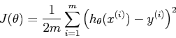
For different values of theta, in this case theta0 and theta1, we can plot the cost function J(theta) in 3d space or as a contour.

j_theta = zeros(250, 250);   % initialize j_theta
theta0_vals = linspace(-5000, 5000, 250);
theta1_vals = linspace(-200, 200, 250);
for i = 1:length(theta0_vals)
   for j = 1:length(theta1_vals)
  theta_val_vec = [theta0_vals(i) theta1_vals(j)]';
  h_theta = (x*theta_val_vec);
  j_theta(i,j) = 1/(2*m)*sum((h_theta - y).^2);
    end
end
figure;
surf(theta0_vals, theta1_vals,10*log10(j_theta.'));
xlabel('theta_0'); ylabel('theta_1');zlabel('10*log10(Jtheta)');
title('Cost function J(theta)');
figure;
contour(theta0_vals,theta1_vals,10*log10(j_theta.'))
xlabel('theta_0'); ylabel('theta_1')
title('Cost function J(theta)');

%linear regression using gradient descent algorithm to find the coefficients, 
%there are many ways to find the coefficients but now we apply gradient descent
%one dimensional data, with an output 
x = load('ex2x.dat');
y = load('ex2y.dat');

figure % open a new figure window
plot(x, y, 'o');
ylabel('Height in meters')
xlabel('Age in years')


m = length(y); % store the number of training examples
x = [ones(m, 1), x]; % Add a column of ones to x
n = size(x,2);
%this part is for minimizing the Theta_vec: coefficients.
theta_vec = [0 0]';
alpha = 0.007;
err = [0 0]';
for kk = 1:10000
 h_theta = (x*theta_vec);
 h_theta_v = h_theta*ones(1,n);
 y_v = y*ones(1,n);
 theta_vec = theta_vec - alpha*1/m*sum((h_theta_v - y_v).*x).';
 err(:,kk) = 1/m*sum((h_theta_v - y_v).*x)';
end

figure;
plot(x(:,2),y,'bs-');
hold on
plot(x(:,2),x*theta_vec,'rp-');
legend('measured', 'predicted');
grid on;
xlabel('x');
ylabel('y');
title('Measured and predicted ');



j_theta = zeros(250, 250);   % initialize j_theta
theta0_vals = linspace(-5000, 5000, 250);
theta1_vals = linspace(-200, 200, 250);
for i = 1:length(theta0_vals)
   for j = 1:length(theta1_vals)
  theta_val_vec = [theta0_vals(i) theta1_vals(j)]';
  h_theta = (x*theta_val_vec);
  j_theta(i,j) = 1/(2*m)*sum((h_theta - y).^2);
    end
end
figure;
surf(theta0_vals, theta1_vals,10*log10(j_theta.'));
xlabel('theta_0'); ylabel('theta_1');zlabel('10*log10(Jtheta)');
title('Cost function J(theta)');
figure;
contour(theta0_vals,theta1_vals,10*log10(j_theta.'))
xlabel('theta_0'); ylabel('theta_1')
title('Cost function J(theta)');

Matlab, Octove or Python for Machine Learning

but  my adviser uses Matlab

I start implementing ML algorithms after learning theory behind them however I really got stuck in which tool to write my code. There are 3 options for now: Octave, Matlab and Python  (read discussions). You can check my previous posts about python, I switched to Python after learning Perl. For now, it seems that for implementation of machine learning algorithms preferring Matlab is a good decision.

There are other tools such as R, Sage etc. i really don't know which one to master, but for now my adviser uses matlab exclusively, so do i.

I list some useful posts that are good when you make your decision :

• Bye Matlab, hello Python, thanks Sage 
• Sage Tour
• R, Octave, and Python: Which Suits Your Analysis Needs?
• Matlab, Python, or R… Time versus Money

Switching From Perl to Python, Step 5 First Step into Machine Learning

in this post i share my experience while searching about the python machine learning modules. There are lots of them, i think that there is no one that can be used for all algorithms, so for a specific algorithm you can choose one of them that satisfies your need.

First i start reading  Scientific Scripting with Python for Computational Immunology, this is the best, short tutorial ever to understand the basic statistics. While going through stackoverflow questions, i realized that many people recommend scikit-learn: machine learning in Python.

i'm familiar with matplotlib and pyplot, however now in examples another module pylab is imported. Clarification: matplotlib, pyplot, and pylab from (http://truongnghiem.wordpress.com):

pyplot is just a wrapper module to provide a Matlab-style interface to matplotlib.

Many plotting functions in Matlab are provided by pyplot with the same names and arguments.

This will ease the process of moving from Matlab to Python for scientific computation.

pylab is basically a mode in which pyplot and numpy are imported in a single namespace,

thus making the Python working environment very similar to Matlab. By importing pylab: 

from pylab import *

we can use Matlab-style commands like:

x = arange(0, 10, 0.2)

y = sin(x)

plot(x, y)

Ok. Let's start, first i try simple linear regression from Scientific Scripting with Python for Computational Immunology. We have dilution.cvs file that contains the data of:

Dilution Factor,Rep 1,Rep 2,Rep 3,Mean,sd
1,15.16,14.95,14.55,14.89,0.31
2,15.36,15.61,15.51,15.49,0.13
4,16.65,16.88,16.71,16.75,0.12
8,18.07,17.60,18.13,17.93,0.29
16,18.86,19.63,19.39,19.29,0.39
32,20.39,19.40,20.39,20.06,0.57
64,21.44,20.76,21.22,21.14,0.35
128,21.90,22.04,21.94,21.96,0.07
256,22.87,22.77,23.36,23.00,0.32
512,23.98,23.92,24.24,24.05,0.17
1024,24.91,24.83,24.92,24.89,0.05
2048,26.37,25.43,26.21,26.00,0.50

Dilution and Factor columns are used in order to implement the linear regression in two dimensional space where the line is defined as :

'''
 *@author beck 
 *@date Sep 14, 2012
 *Basic Statistics with Python 
 *bekoc.blogspot.com 
'''

import numpy
import matplotlib.pyplot as plt
#import pylab, # from pylab import *
import scipy.stats as stats

xs= numpy.loadtxt("dilution.csv",delimiter=",", skiprows=1, usecols=(0,1)) 

# numpy array - similar to C array notation.
x= numpy.log2(xs[:,0])
y=xs[:,1]

plt.plot(x,y,"x")
        
plt.xlabel('Number of Dilutions(log2)')
plt.ylabel('Rep1')
plt.title('Linear Regression example')
plt.legend()

slope, intercept, r_value, p_value, std_error = stats.linregress(x,y)
plt.plot(x,intercept+slope*x,"r-") # y=mx+b where m is slope and b is intercept
#plt.plot(x,x**2)
plt.show()

straight line seems reasonable

Resources for machine learning:

scikit-learn: machine learning in Python, Easy-to-use and general-purpose machine learning in Python

Is there a recommended package for machine learning in Python?

Switching From Perl to Python, Step 4 Basic Statistics

On August 28 2012 at 10am, the creator of matplotlib, John D. Hunter died from complications arising from cancer treatment, after a brief but intense battle with this terrible illness. John is survived by his wife Miriam, his three daughters Rahel, Ava and Clara, his sisters Layne and Mary, and his mother Sarah. If you have benefited from John's many contributions, please say thanks in the way that would matter most to him. Please consider making a donation to the John Hunter Memorial Fund.

Rest in peace, John  Hunter (1968-August 28th, 2012). My sincere condolences to his family. Thank you for all your contribution. A great loss to the community.Thank you again.  

After learning the basics of Python, today i will try to implement some basic statistical methods including plotting. We need two important packages mathplotlib and scipy. I remember that there is also numpy library, a bit confused but it's explained very well in official scipy documentation:

"SciPy (pronounced "Sigh Pie") is open-source software for mathematics, science, and engineering. It is also the name of a very popular conference on scientific programming with Python. The SciPy library depends on NumPy, which provides convenient and fast N-dimensional array manipulation. The SciPy library is built to work with NumPy arrays, and provides many user-friendly and efficient numerical routines such as routines for numerical integration and optimization."

i follow two useful blogs in order to learn how to plot and make basic statistical calculation by using pyton, after i learn these topics, i will search about machine learning libraries.

• Simple statistics with SciPy
• Basic Data Plotting with Matplotlib Part 3: Histograms

Switching From Perl to Python, Step 3 Python Data Structures

We read the Knuth, so you don't need to

-Tim Peters

After finishing first part of Python, today i decided to read about Python data structures.
Today's topics are:
Night -2-
10.  Modules
11.  Data Structures
12.  Problem Solving

While i was reading about the data structures in Python, list, tuple and dictionary implementations are very similar to corresponding Java collections list, set and map. Please check here to review some examples.

While reading about the dictionaries, defaultdict implementation was interesting, in addition, i really like the one liners, as an example:

myfile=open('names', 'r')
words=[line.rstrip() for line in myfile]
quote='''google
        excite
        yahoo
        bing
        altavista '''
#find the words that exits in file but not in quote
difference=[word for word in quote.split() if word not in words]
print difference

Some useful resources:
Python in High performance computing 
Official python documentation
Data Structures and Algorithms Using Python

Switching From Perl to Python, Step 2 Python Basics

 If you don't know any computer languages, I recommend starting with Python. It is cleanly designed, well documented, and relatively kind to beginners. Despite being a good first language, it is not just a toy; it is very powerful and flexible and well suited for large projects.

How To Become A Hacker, Eric Steven Raymond

From coffeeghost

Following topics are from Byte of Python which is a free Python book for completely beginners.
Today's topics:

Night -1-
1. → Translations
2. → Preface
3. → Introduction
4. → Installation
5. → First Steps
6. → Basics
7. → Operators and Expressions
8. → Control Flow
9. → Functions 

Resources that i have reviewed:

• http://wiki.python.org/moin/SimplePrograms
• http://www.sthurlow.com/python/
• http://cs.simpson.edu/?q=node/26 : when i was reading this page, Pygame Graphics Examples were interesting

Switching From Perl to Python, Step 1 Which IDE to use for Python programming ?

 Python 2.x is the status quo, Python 3.x is the present and future of the language (http://wiki.python.org/moin/Python2orPython3)

i followed the instruction from vogella, however instead of installing python 2.7 directly from official python web page, i installed from enthought academic version which includes the numpy, Scipy and matplotlib. These modules will be useful when we start programming,
i do not give details for now.

Academic versions of Enthought:
Students or employees from degree-granting institutions may use these installations for an extended period free of cost.

After installing Eclipse and configuration of PyDev , i guess i'm ready for Python. Actually, i'd like to use netbeans instead but netbeans does not have python support after 7.0 versions.

Some experiments to be sure that everything works smoothly:

1-First (little) Python module (from vogella)

2- First (little)NumPy module

3-Scipy and Matplotlib module

Code is from oneau

Ok. then i'm ready for Night 1 for tomorrow:

1. → Translations
2. → Preface
3. → Introduction
4. → Installation
5. → First Steps
6. → Basics
7. → Operators and Expressions
8. → Control Flow
9. → Functions